interval estimation HistFactory-style¶

The HistFactory p.d.f. template [CERN-OPEN-2012-016] is per-se independent of its implementation in ROOT and sometimes, it’s useful to be able to run statistical analysis outside of ROOT, RooFit, RooStats framework.

This repo is a pure-python implementation of that statistical model for multi-bin histogram-based analysis and its interval estimation is based on the asymptotic formulas of “Asymptotic formulae for likelihood-based tests of new physics” [arXiv:1007.1727]. The aim is also to support modern computational graph libraries such as PyTorch and TensorFlow in order to make use of features such as autodifferentiation and GPU acceleration.

Hello World¶

This is how you use the pyhf Python API to build a statistical model and run basic inference:

>>> import pyhf
>>> model = pyhf.simplemodels.hepdata_like(signal_data=[12.0, 11.0], bkg_data=[50.0, 52.0], bkg_uncerts=[3.0, 7.0])
>>> data = [51, 48] + model.config.auxdata
>>> test_mu = 1.0
>>> CLs_obs, CLs_exp = pyhf.infer.hypotest(test_mu, data, model, qtilde=True, return_expected=True)
>>> print(f"Observed: {CLs_obs}, Expected: {CLs_exp}")
Observed: 0.05251497423736956, Expected: 0.06445320535890459

Alternatively the statistical model and observational data can be read from its serialized JSON representation (see next section).

>>> import pyhf
>>> import requests
>>> wspace = pyhf.Workspace(requests.get('https://git.io/JJYDE').json())
>>> model = wspace.model()
>>> data = wspace.data(model)
>>> test_mu = 1.0
>>> CLs_obs, CLs_exp = pyhf.infer.hypotest(test_mu, data, model, qtilde=True, return_expected=True)
>>> print(f"Observed: {CLs_obs}, Expected: {CLs_exp}")
Observed: 0.3599840922126626, Expected: 0.3599840922126626

Finally, you can also use the command line interface that pyhf provides which should produce the following JSON output:

$ cat << EOF  | tee likelihood.json | pyhf cls
{
    "channels": [
        { "name": "singlechannel",
          "samples": [
            { "name": "signal",
              "data": [12.0, 11.0],
              "modifiers": [ { "name": "mu", "type": "normfactor", "data": null} ]
            },
            { "name": "background",
              "data": [50.0, 52.0],
              "modifiers": [ {"name": "uncorr_bkguncrt", "type": "shapesys", "data": [3.0, 7.0]} ]
            }
          ]
        }
    ],
    "observations": [
        { "name": "singlechannel", "data": [51.0, 48.0] }
    ],
    "measurements": [
        { "name": "Measurement", "config": {"poi": "mu", "parameters": []} }
    ],
    "version": "1.0.0"
}
EOF
{
   "CLs_exp": [
      0.0026062609501074576,
      0.01382005356161206,
      0.06445320535890459,
      0.23525643861460702,
      0.573036205919389
   ],
   "CLs_obs": 0.05251497423736956
}

What does it support¶

Implemented variations:

☑ HistoSys
☑ OverallSys
☑ ShapeSys
☑ NormFactor
☑ Multiple Channels
☑ Import from XML + ROOT via uproot
☑ ShapeFactor
☑ StatError
☑ Lumi Uncertainty

Computational Backends:

☑ NumPy
☑ PyTorch
☑ TensorFlow
☑ JAX

Optimizers:

☑ SciPy (scipy.optimize)
☑ MINUIT (iminuit)

All backends can be used in combination with all optimizers. Custom user backends and optimizers can be used as well.

Todo¶

☐ StatConfig
☐ Non-asymptotic calculators

results obtained from this package are validated against output computed from HistFactory workspaces

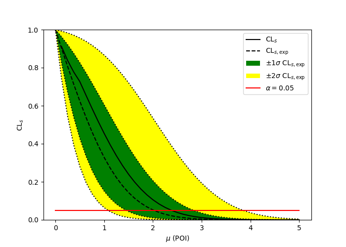
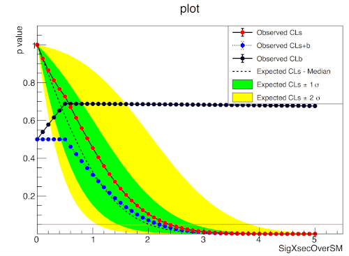
A one bin example¶

import pyhf
import numpy as np
import matplotlib.pyplot as plt
import pyhf.contrib.viz.brazil

pyhf.set_backend("numpy")
model = pyhf.simplemodels.hepdata_like(
    signal_data=[10.0], bkg_data=[50.0], bkg_uncerts=[7.0]
)
data = [55.0] + model.config.auxdata

poi_vals = np.linspace(0, 5, 41)
results = [
    pyhf.infer.hypotest(test_poi, data, model, qtilde=True, return_expected_set=True)
    for test_poi in poi_vals
]

fig, ax = plt.subplots()
fig.set_size_inches(7, 5)
ax.set_xlabel(r"$\mu$ (POI)")
ax.set_ylabel(r"$\mathrm{CL}_{s}$")
pyhf.contrib.viz.brazil.plot_results(ax, poi_vals, results)

pyhf

ROOT

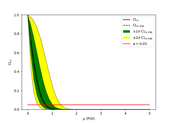
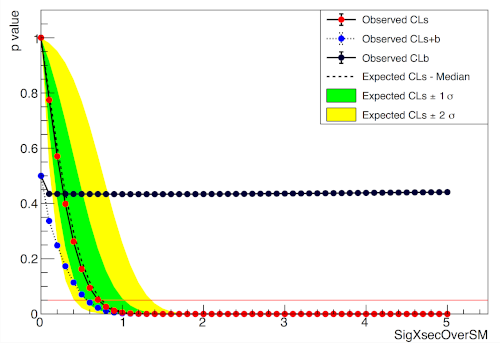
A two bin example¶

import pyhf
import numpy as np
import matplotlib.pyplot as plt
import pyhf.contrib.viz.brazil

pyhf.set_backend("numpy")
model = pyhf.simplemodels.hepdata_like(
    signal_data=[30.0, 45.0], bkg_data=[100.0, 150.0], bkg_uncerts=[15.0, 20.0]
)
data = [100.0, 145.0] + model.config.auxdata

poi_vals = np.linspace(0, 5, 41)
results = [
    pyhf.infer.hypotest(test_poi, data, model, qtilde=True, return_expected_set=True)
    for test_poi in poi_vals
]

fig, ax = plt.subplots()
fig.set_size_inches(7, 5)
ax.set_xlabel(r"$\mu$ (POI)")
ax.set_ylabel(r"$\mathrm{CL}_{s}$")
pyhf.contrib.viz.brazil.plot_results(ax, poi_vals, results)

pyhf

ROOT

Installation¶

To install pyhf from PyPI with the NumPy backend run

python -m pip install pyhf

and to install pyhf with all additional backends run

python -m pip install pyhf[backends]

or a subset of the options.

To uninstall run

python -m pip uninstall pyhf

Questions¶

If you have a question about the use of pyhf not covered in the documentation, please ask a question on Stack Overflow with the [pyhf] tag, which the pyhf dev team watches.

If you believe you have found a bug in pyhf, please report it in the GitHub Issues. If you’re interested in getting updates from the pyhf dev team and release announcements you can join the pyhf-announcements mailing list.

Citation¶

As noted in Use and Citations, the preferred BibTeX entry for citation of pyhf is

@software{pyhf,
  author = "{Heinrich, Lukas and Feickert, Matthew and Stark, Giordon}",
  title = "{pyhf: v0.5.3}",
  version = {0.5.3},
  doi = {10.5281/zenodo.1169739},
  url = {https://github.com/scikit-hep/pyhf},
}

Authors¶

pyhf is openly developed by Lukas Heinrich, Matthew Feickert, and Giordon Stark.

Please check the contribution statistics for a list of contributors.

Milestones¶

2020-07-28: 1000 GitHub issues and pull requests. (See PR #1000)

Acknowledgements¶

Matthew Feickert has received support to work on pyhf provided by NSF cooperative agreement OAC-1836650 (IRIS-HEP) and grant OAC-1450377 (DIANA/HEP).